Prototyping (June 2025)

An evolution of prototyping.

Prototype #1

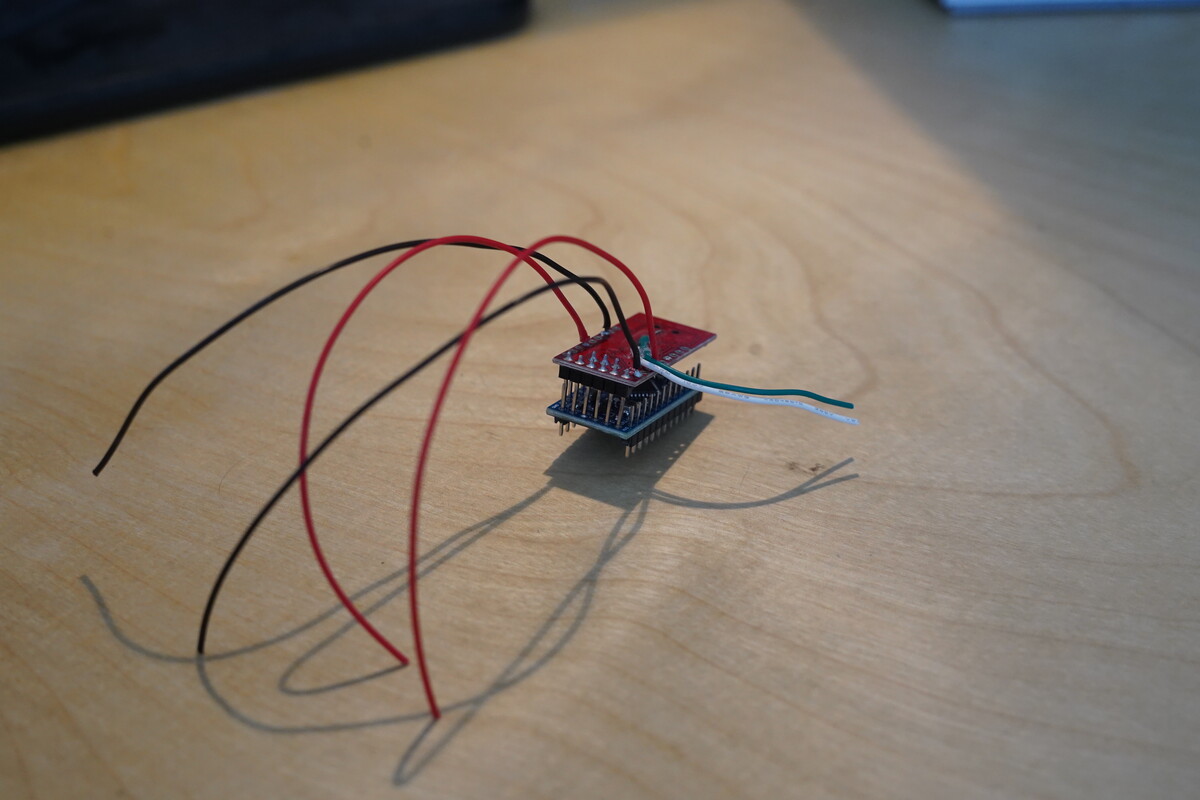
The blue board is an Arduino mini pro 3v3. The red board is an FTDI 232RL USB<->UART board.

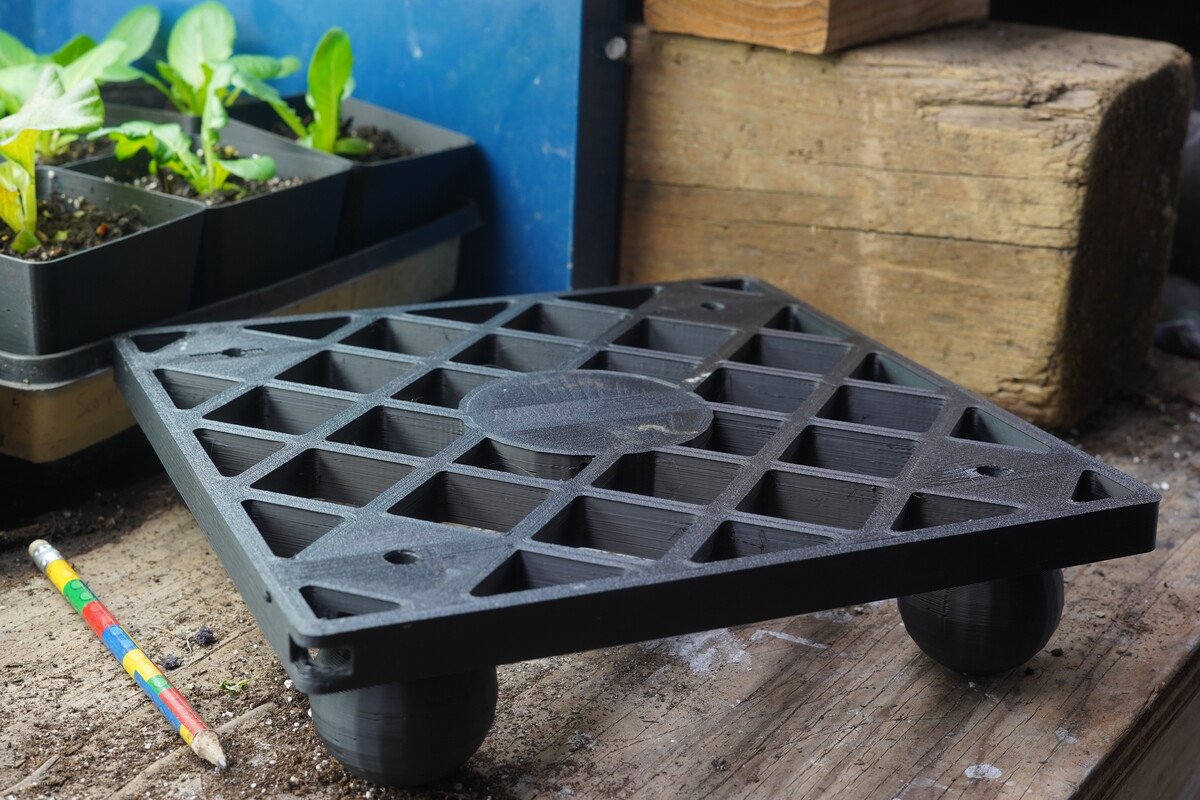
The first prototype. Load cells and electronics mounted to the bottom of 10”x20” gardening tray.

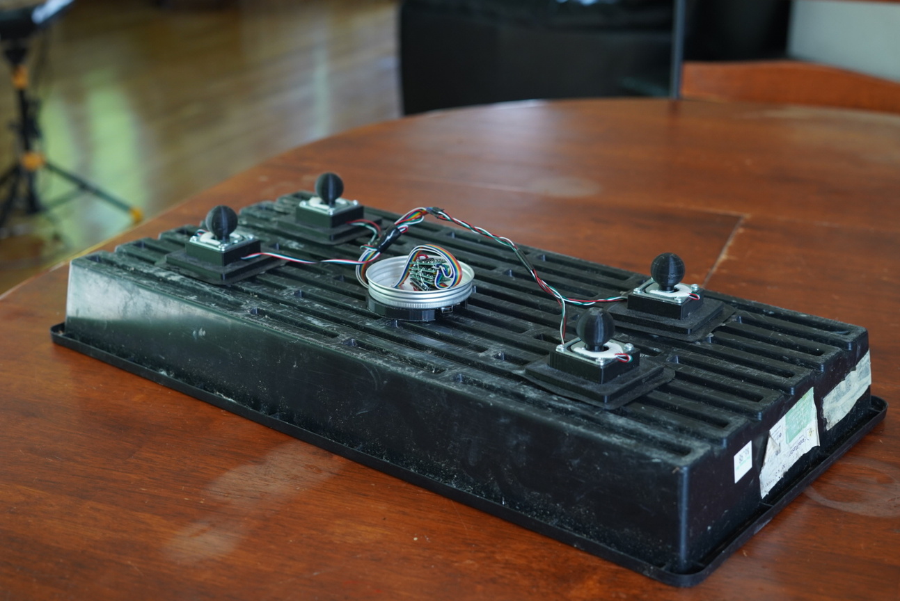
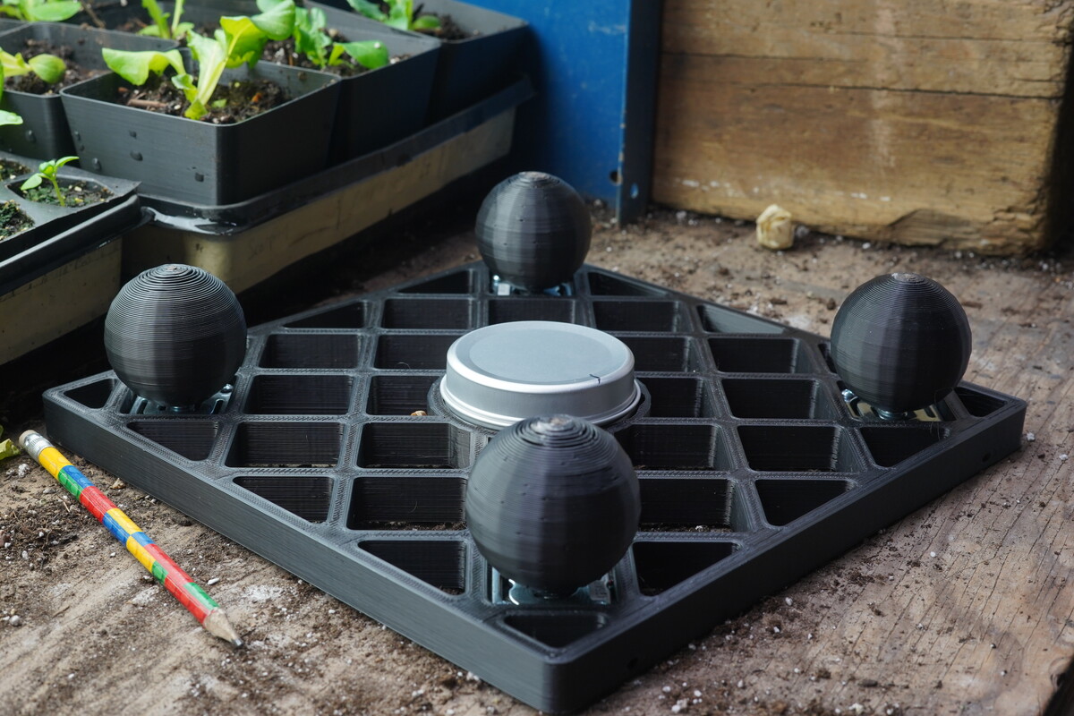
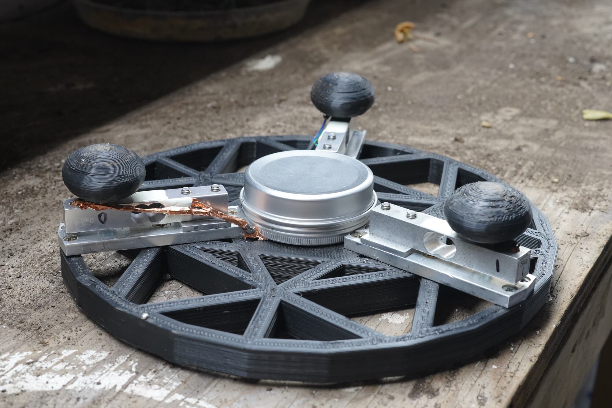
Shown here is a spherical foot, a load cell and a mounting plate on the bottom of a gardening tray.

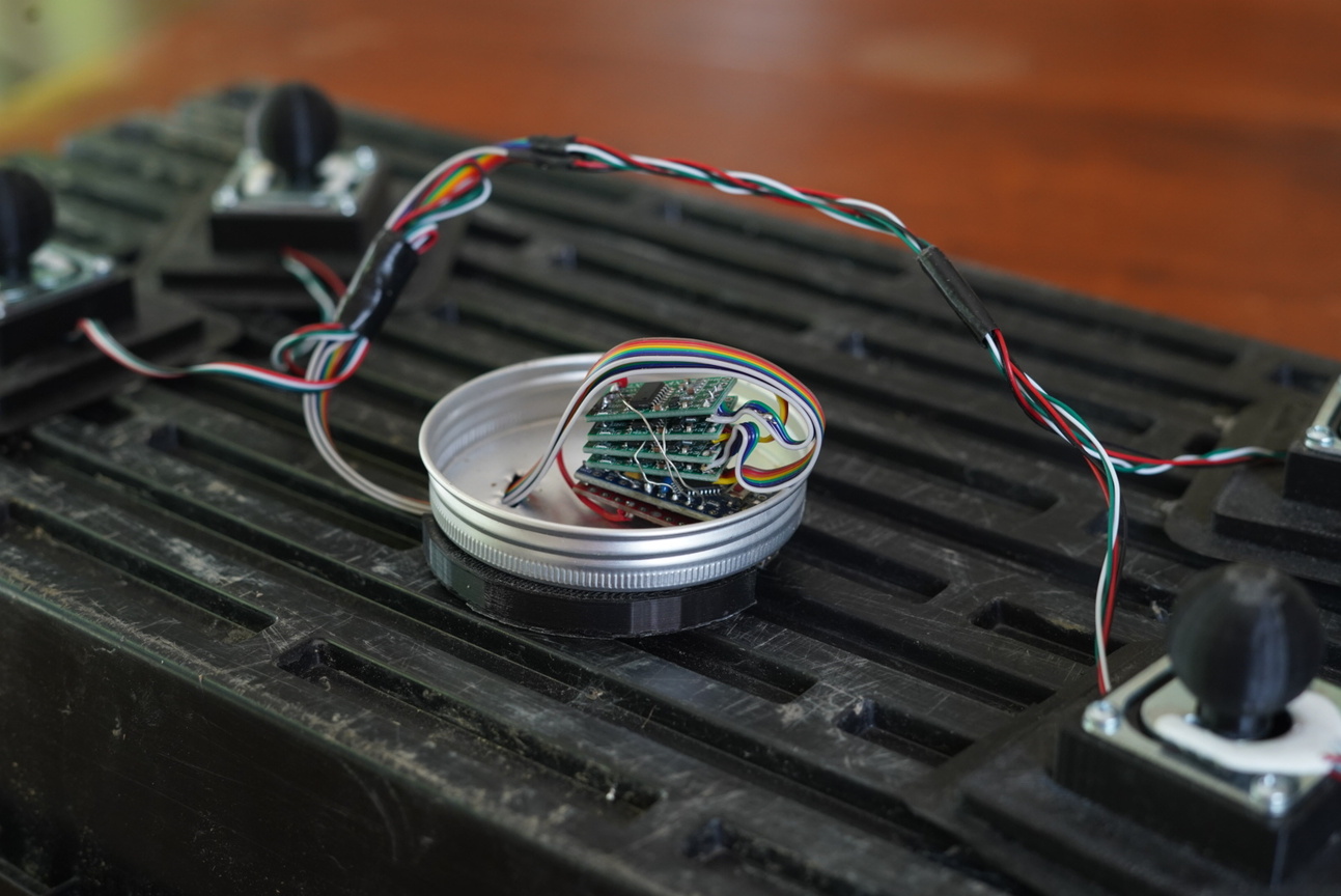
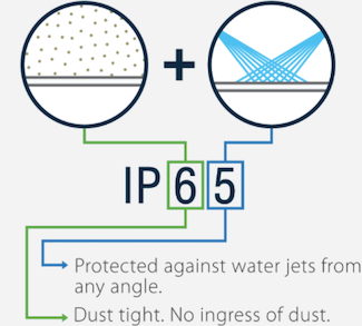
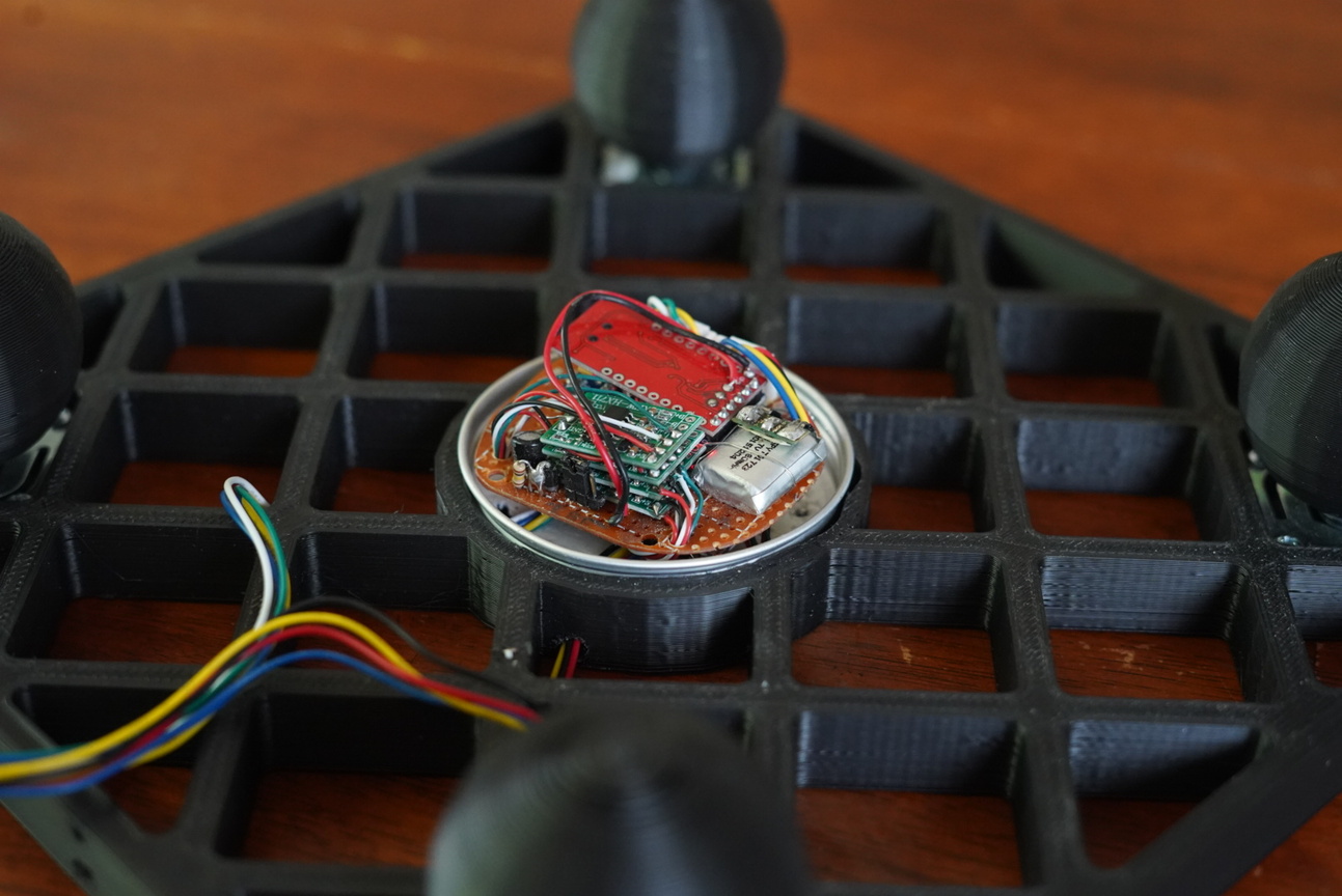
The electronics go into a 2 ounce tin for electromagnetic interference and dust/spray protection. I am going for IP65 rating.

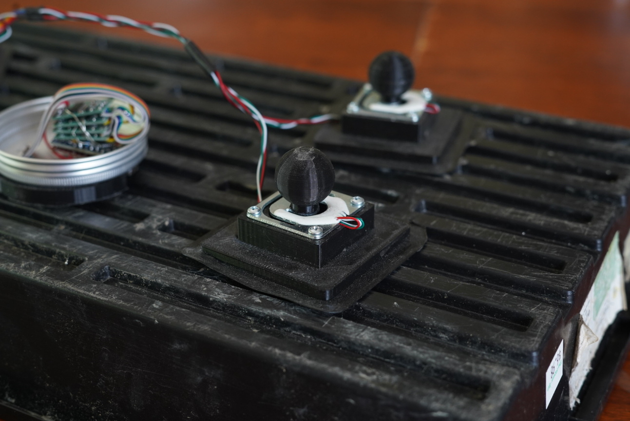
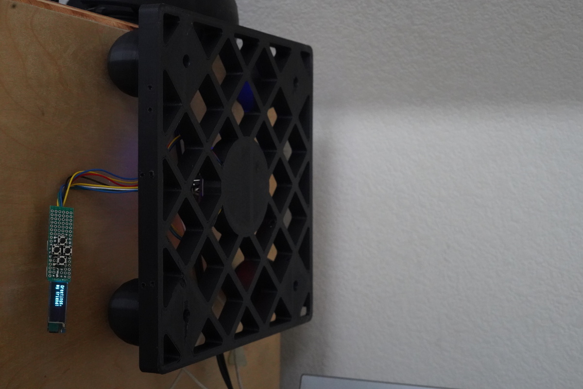
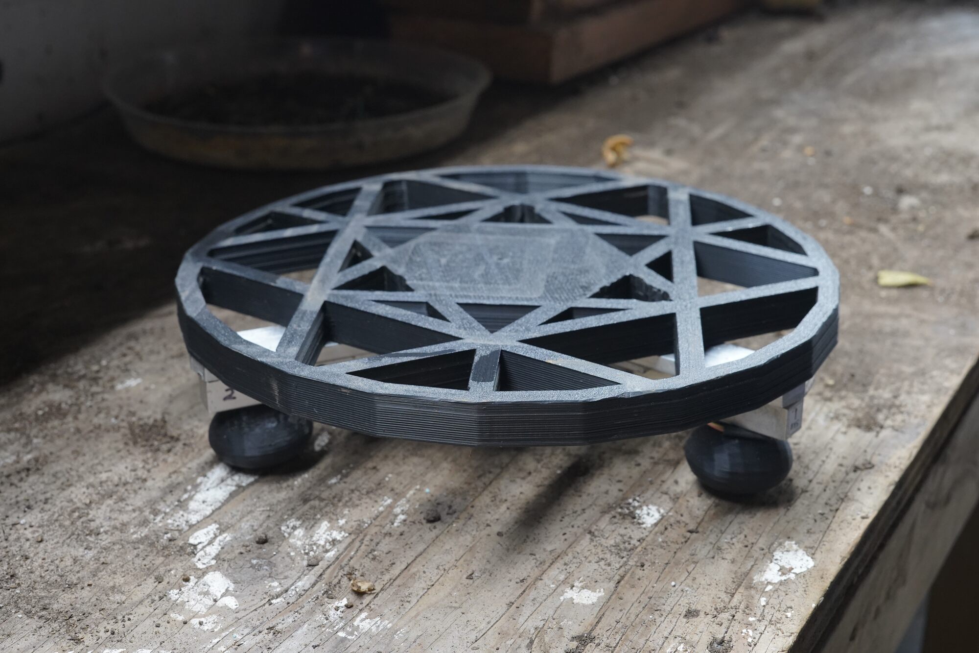
This is the first 3D-printed prototype. The spherical feet are to better float on soft terrain, such as pea gravel. The wiring to the load sensors passes through the frame.

The electronics go inside the 2 ounce tin.

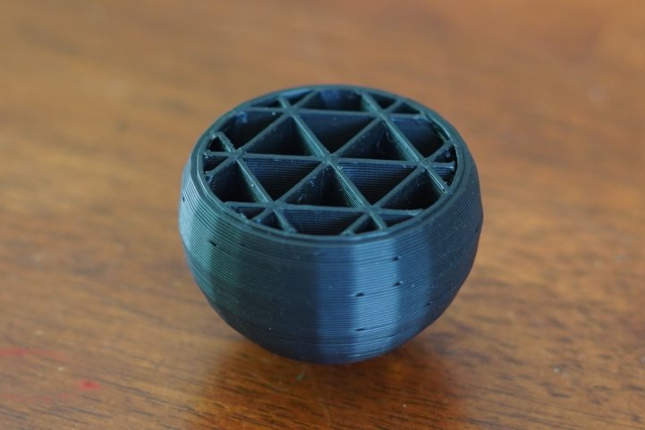
It was fun getting the 3D printing fill to work good with a sphere.

Growing lettuce.

Controls and a display were added. Unfortunately, the microcontroller was accidentally destroyed before the LCD display could be made functional.

Prototype #2

Functional OLED LCD. Simplified controls.

The electronics:

• Arduino mini pro 3v3

• FTDI 232RL USB <-> UART

• 4x HX711

• TP4056 power charging and protection

• 180mA battery

Testing

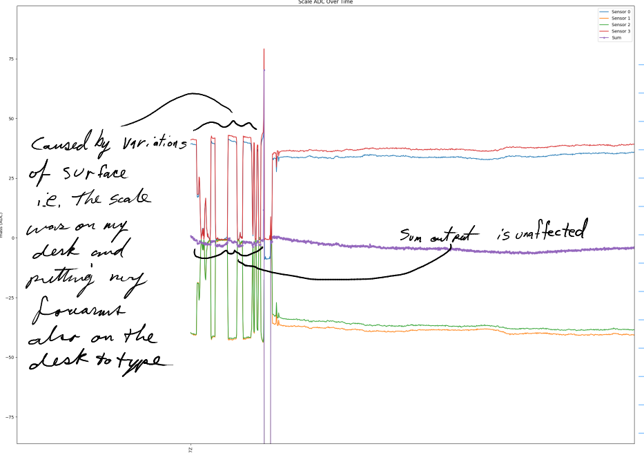
#1: Zero Offset Drift - Initial

This is some zero offset drift testing showing 120g of drift over about 11 hours. That’s not good, I am engineering to +/- 5g for the long term time range.

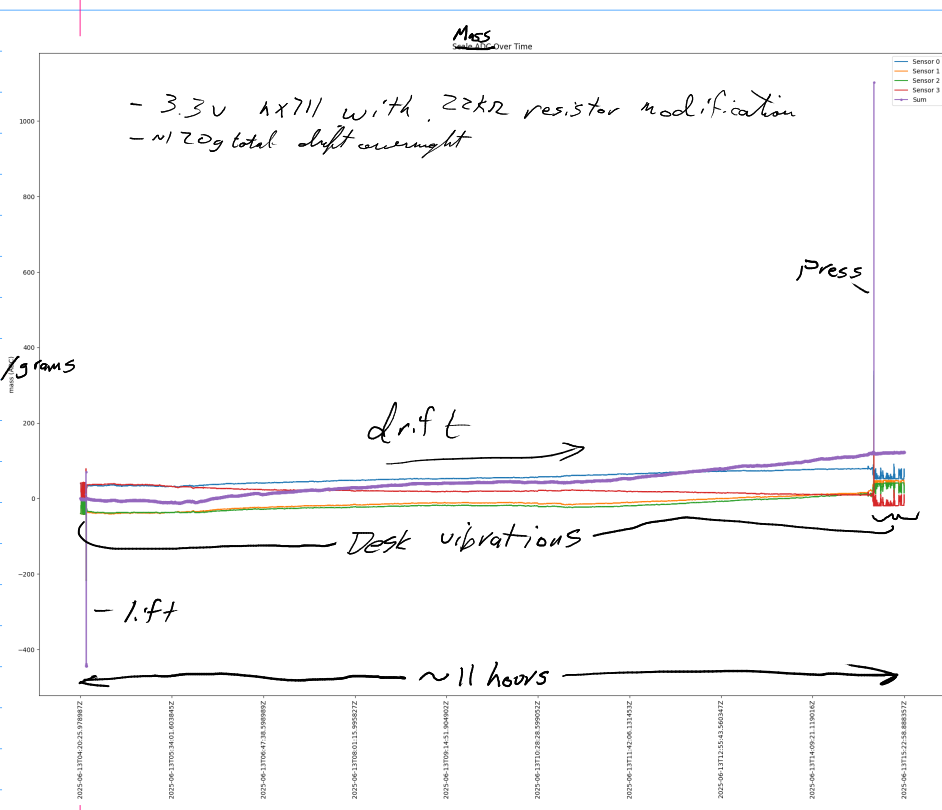
The good news is that the short term time range is very sensitive with good resolution. This is great for manual/automated watering use cases.

Also good news is that the summing of the independent scales makes the mass output more immune to environmental vibrations when compared to a distributed bridge scale architecture.

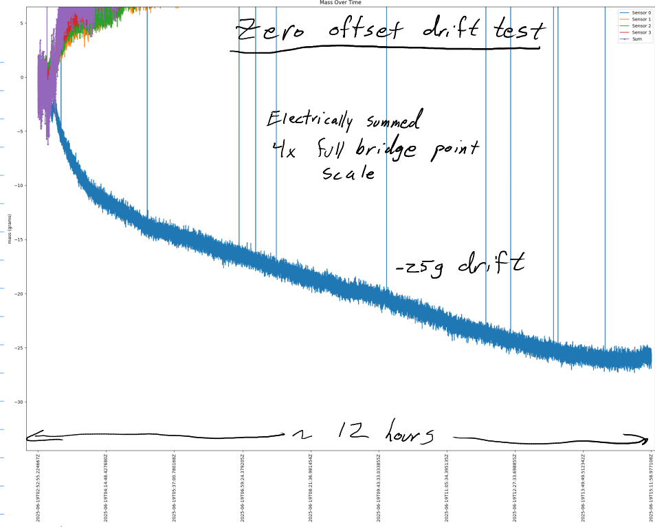
#2: Zero Offset Drift - Longer time

More zero offset drift testing was performed. Still at 3.3V running to modified hx711 boards for 2.7v excitation.

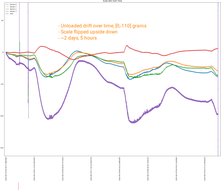
Loaded drift testing.

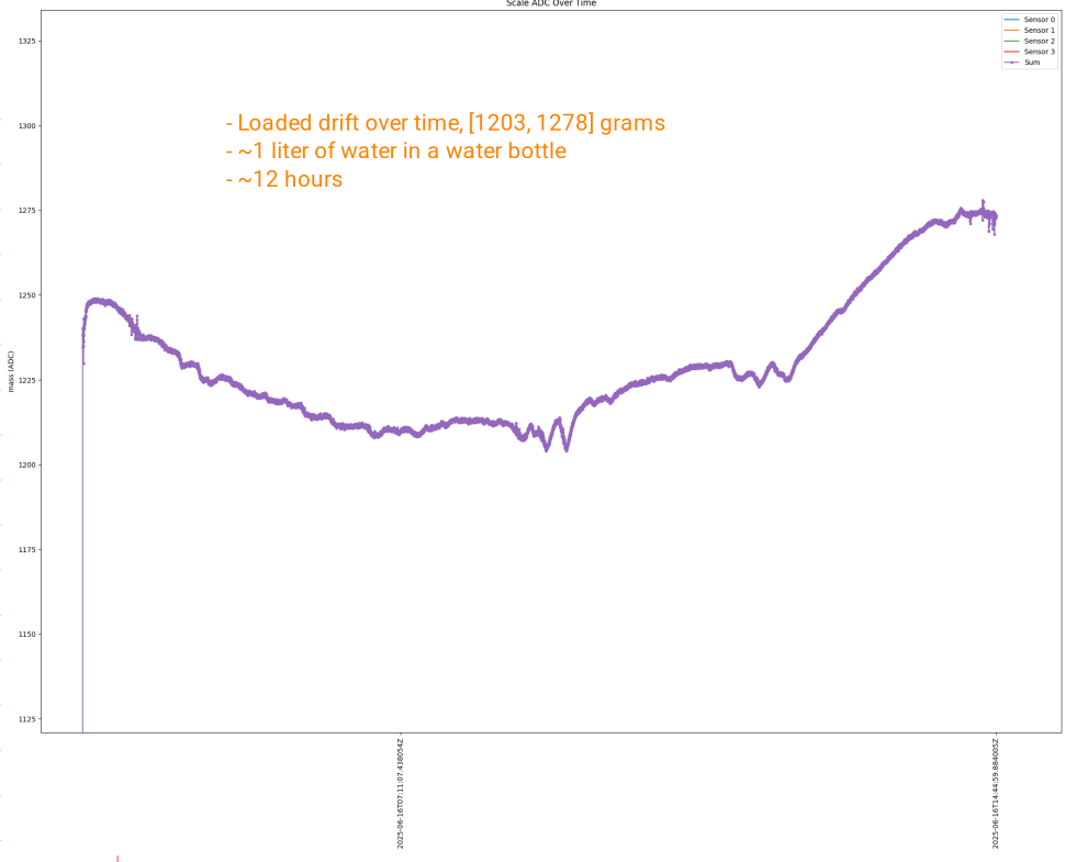
These results were not good. The goal is for the error to not exceed +/- 5g due to drifting.

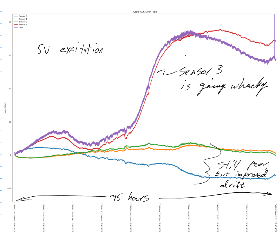
#3: 5v Drift

The load cell excitation voltage was increased from 2.7v to 4.2v. Some improvement observed in zero offset drift for sensors 0,1 & 2. Sensor 3 is going way out of bounds.

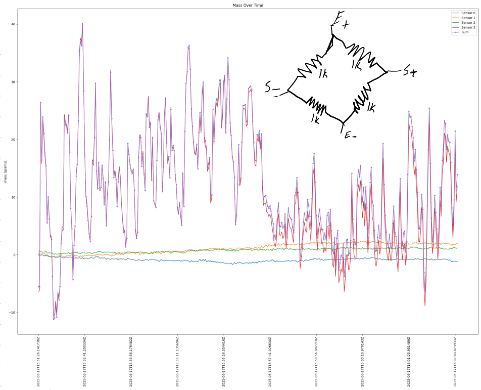
#4: Op-amp & ADC Check

In this test, the mass sensing is simplified to these four parts:

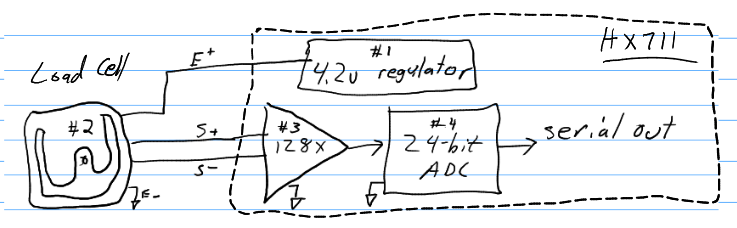
• #1: A voltage regulator driving the load cell sensor(s). There is an onboard 4.2 voltage regulator included with the hx711 board.

• #2: A load cell, please excuse the poor drawing :)

• #3: Programmable gain op-amps. In this testing, only channel A, gain 128x is being tested.

• #4: A 24bit digital to analog converter output to bit-banging serial.

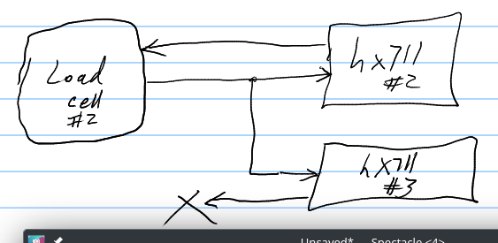
I would like to know what is wrong on with sensor #3. The four components were dissected in half. This was accomplished by

• disconnecting sensor #3’s load cell

• connect sensor #2 load cell output to sensor #2 & #3 hx711 input.

Shown below:

Here are the results:

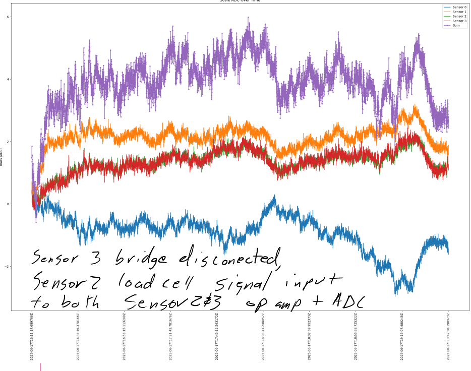
The sensor 3 data matches sensor 2 data very well. This means that sensor 3 op amp & ADC are functioning the same as sensor 2’s. It is unlikely that both sensor’s op-amp & ADC would be bad and behave identically, so assume that sensor 2 & 3’s op-amp & ADC are functioning properly.

This indicates that the problem is in sensor #3’s voltage regulator or load cell.

#5: 1k ohm Resistor Wheatstone Bridge Stand-in

A wheatstone bridge was built out of four 1k ohm resistors. It was then used in place of a load cell for sensor #3.

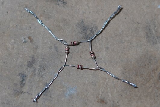
The results were interesting. This is the first time I have tried to use static resistors as a stand in for a load cell. I’m not sure what to make of the data other than sensor #3 behaved erratically.

#6: Parallel HX711 Voltage Regulators

Next, the voltage regulators of all hx711 boards were ran in parallel.

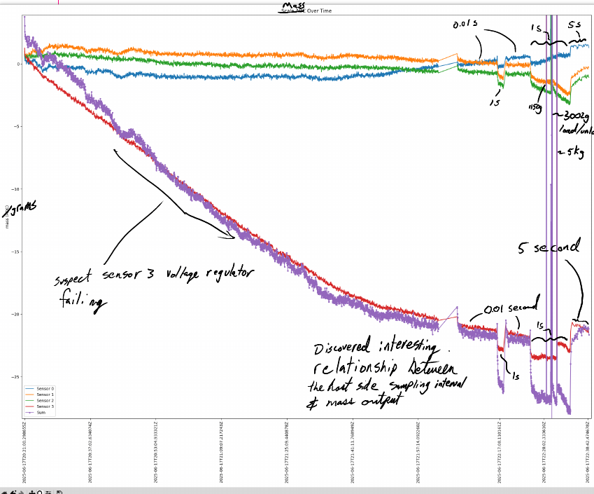
The drift of sensor 0,1 & 2 looks good. Sensor 3 does not. I suspect the voltage regulator of the sensor 3 hx711 board is failing.

Secondary observations were made. A DC shift can be introduced through changes in the host sampling interval, loading/unloading the scale and turning the power on/of between host samples. All of these are likely due to heating, either in the HX711 board or in the load cell strain gages.

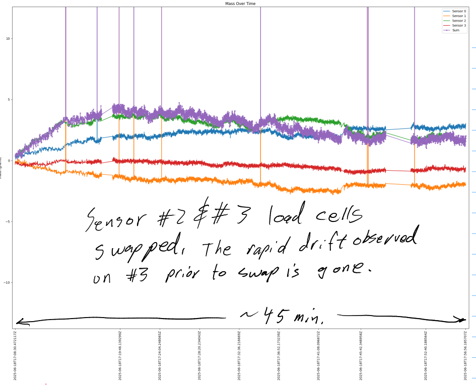
#7: Cross-swap Sensor #2 & #3 load cells

The steep drift observed with sensor #3 stopped when sensor #2 & #3 load cells were swapped. Additionally, no problem found on sensor #2 with sensor #3’s load cell.

Noise observed on sensor 1.

#8: Attempt to Repeat #6

The cross-swap from #7 was reverted. The attempt repeat the bad drift on sensor #3 observed in test #6 was made. The problem did not repeat.

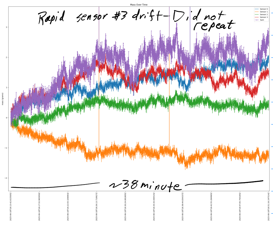
I am not sure why the problem did not repeat. My leading hypothesis is a floating ground that was fixed during the cross-swap experiment.

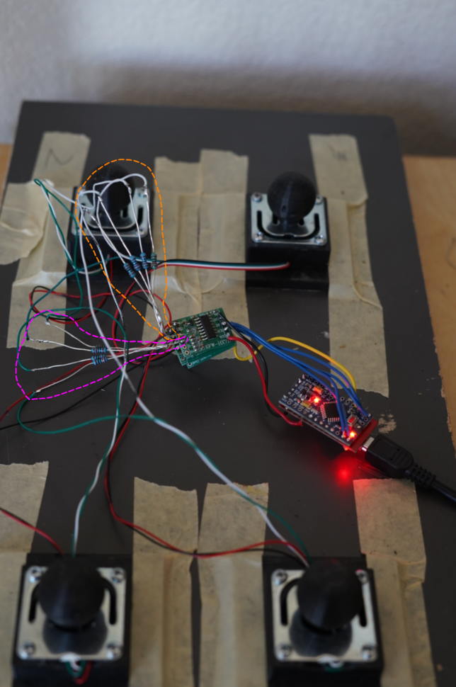
#9: Electrically Sum Load Cells

Here, a single HX711 board is used with the load cell differential signals electrically summed, using an adder circuit.

Reference

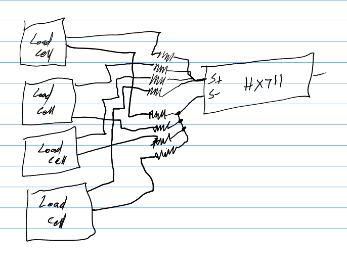
For four wheatstone bridge sensors and from experimentation, the resistors shown above and in the schematic were not needed.

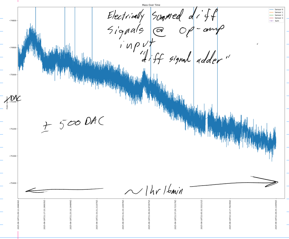
Here is a longer test of the drift.

#10: AC Excitation

In this experiment, AC excitation as added. Similiar to experiment #9, 4x full bridge load cells were used along with a single HX711 board, where the signals are electrically summed at the op-amp input.

A maximum drift of 31g was observed over 36 hours.

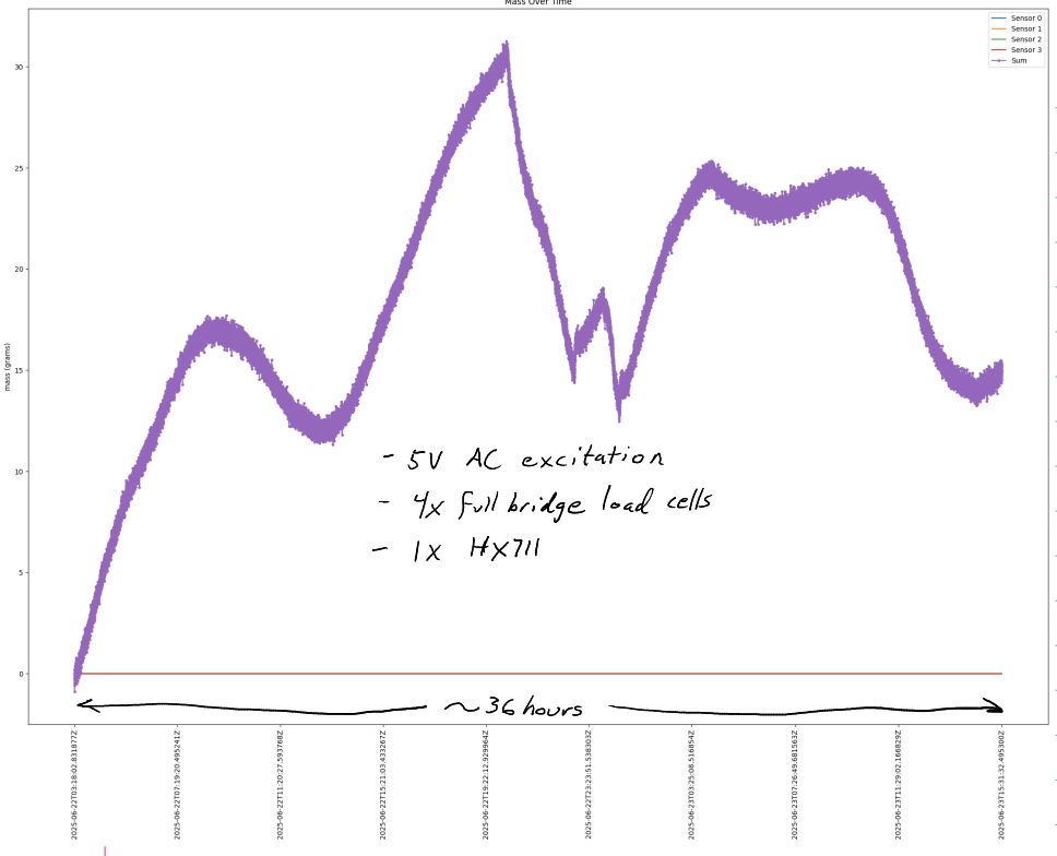
I was hoping for more drift removal than what was observed. I suspect that the AC excitation is removing thermal drift from the strain gages. I suspect that the remaining observed drift is largely made up of physical deformation of the load cells due to temperature.

References:

• Texas Instruments - A Basic Guide to Bridge Measurements

• Texas Instruments - Reduce Bridge Measurement Offset and Drift Using AC Excitation Mode

#12: Temperature HX711 Channel B

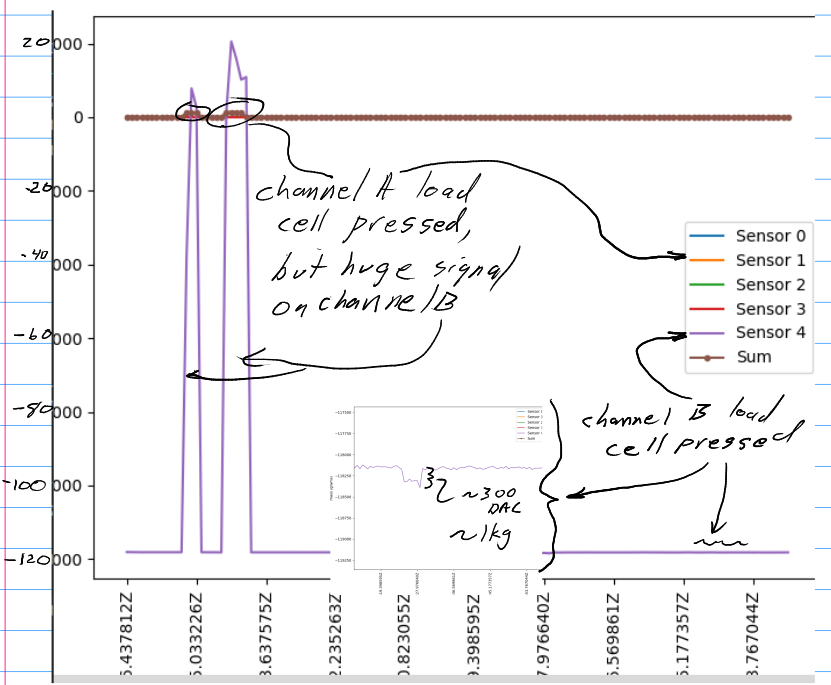
A load cell was wired to sensor #1’s HX711 channel B input. The load cell was mounted in a way to minimize any stress induced variances. With this, it is intended to serve as a temperature reference for the weigh scale.

Here is the hardware configuration:

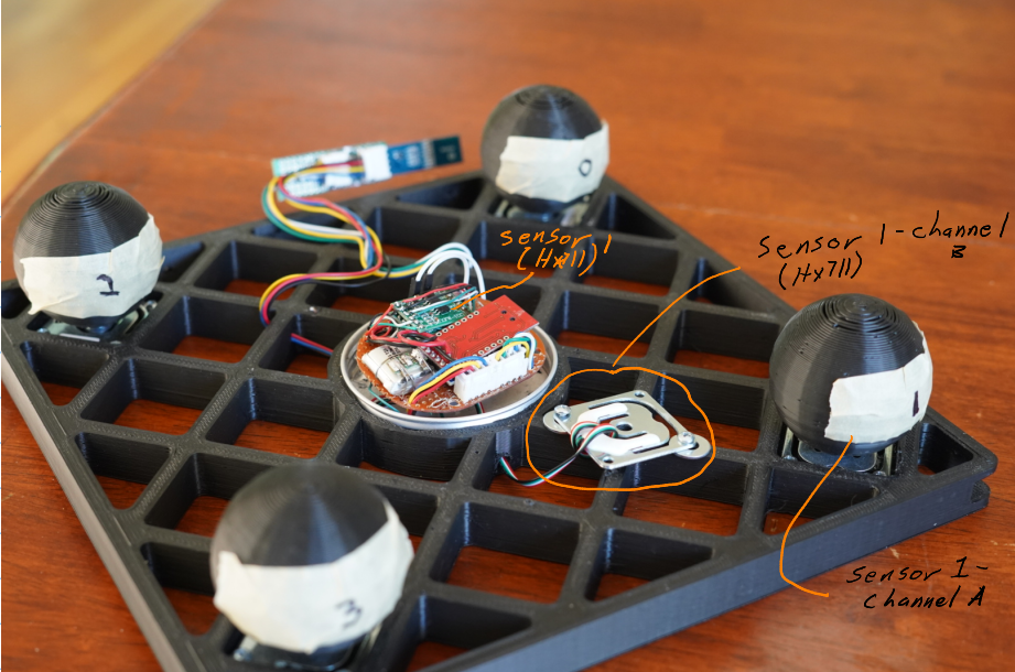
A problem was encountered in which the channel A signal was affecting the channel B signal. In fact, the signal from A was greater, by orders of magnitude, than the approximately 1kg load placed on the channel B load cell.

#13: Temperature with Dedicated HX711

The same hardware was used from experiment #12. This time, The four load cells were summed electrically at the input of sensor 1. The reference temperature load cell was input to its own HX711 board, sensor 0.

The fixture was placed on a 3D printer heat bed. The temperature was cycle between approximately 22*C and 50*C.

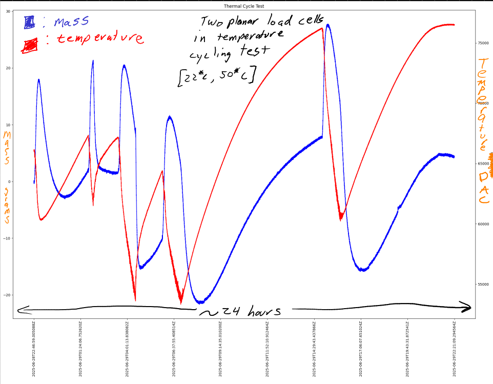
Here is a temperature (DAC) vs mass (grams) plot. Whoa, that’s a pretty cool plot. That’s all sorts of unpredictable though. I don’t think it will be practical to use an auxiliary load cell for temperature sensing.

#14: Mass & Temperature Planar Load Cell

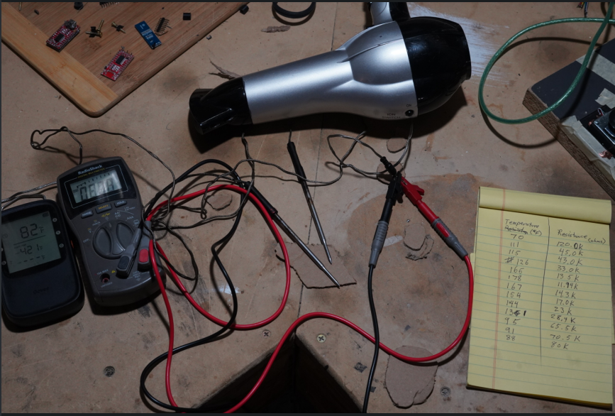
A meat thermometer was used as a temperature sensor in an attempt to correlate temperature with mass.

First, the resistance/temperature response needed to be determined for the temperature probe.

Next, the temperature vs. resistance is plotted and a line of best fit analysis is made.

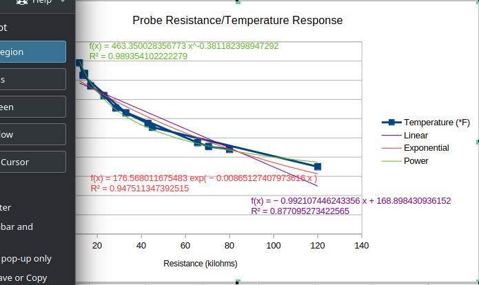
From the R^2 value, it looks like the power curve fits the best.

The probe was then put into a voltage divider circuit, shown in the circuit as R2. R2 represents the temperature probe.

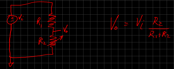
R1 needs to be selected in a way to most fully use the Arduino analog input range [0,3.3] volts in this case.

40 kohm was chosen. I think the the closest I had on hand was 44 kohm or so.

Finally, the same correlation was made, except this time temperature *F vs. digital to analog converted (DAC) value.

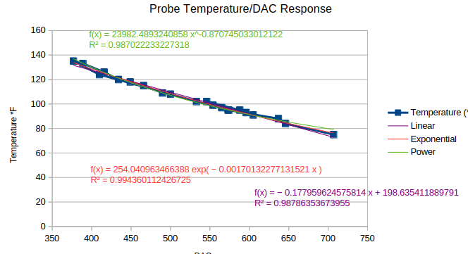
This time R^2 shoes a linear fit to be best. Placing the probe into a voltage divider linearized the output, sweet!

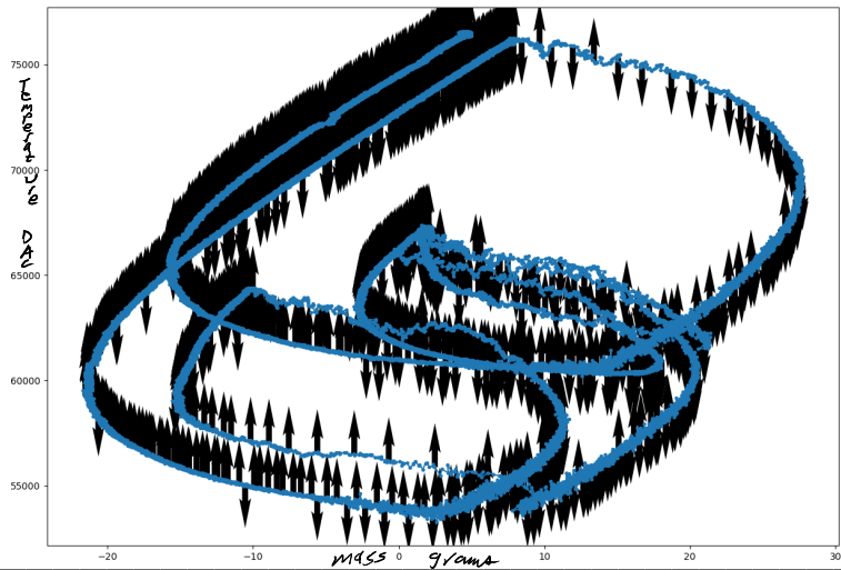
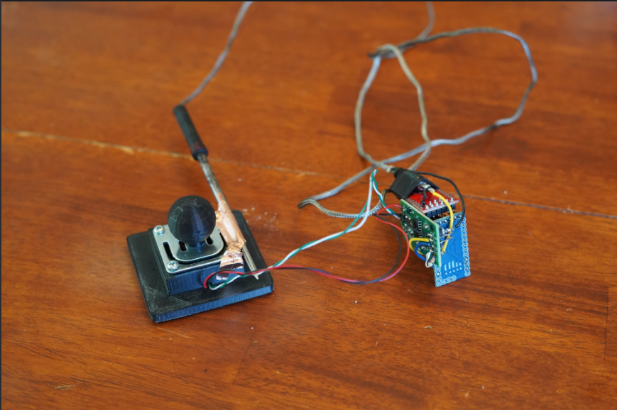
Here is the fixture for mass & temperature over time for an unloaded planar, full-bridge load cell.

3x thermal cycling [22*C, 50*C] test data:

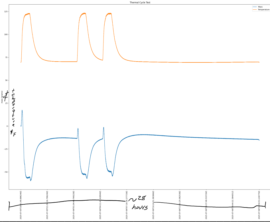
The total change in mass was about (-60, 20) grams.

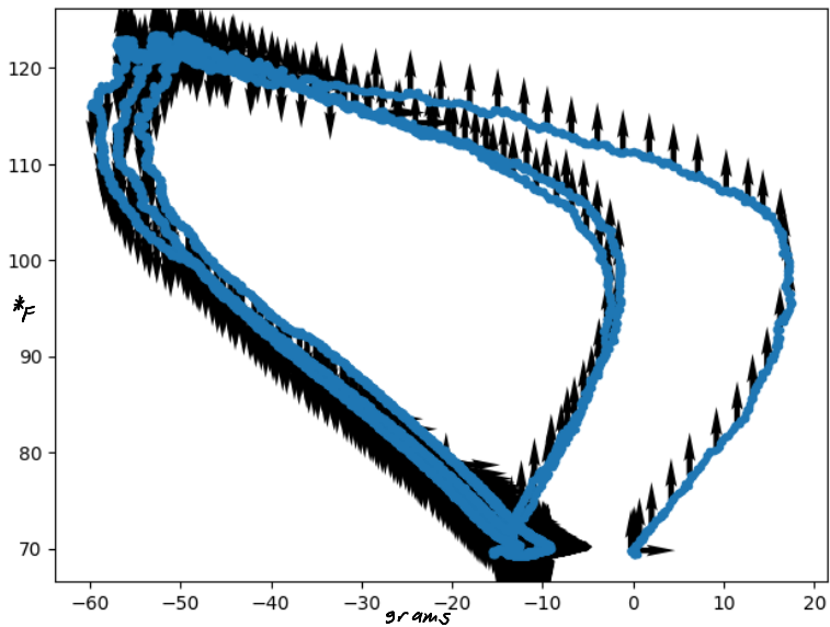
The arrows in the plat above indicate which direction the temperature is going. There is hysteresis when going up/down in temperature. There are also hystereses observed when going in just one direction in temperature. The width of the hysteresis was 80 grams.

The implications of this is that the mass of something being weighed can only be known to [-60, 20] grams. It would be difficult to correct the mass output with temperature sensing due to the multiple hystereses and general non-repeatable nature.

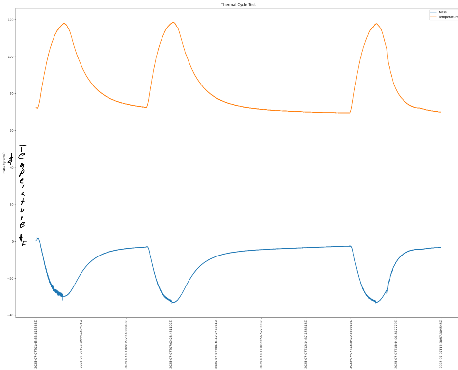
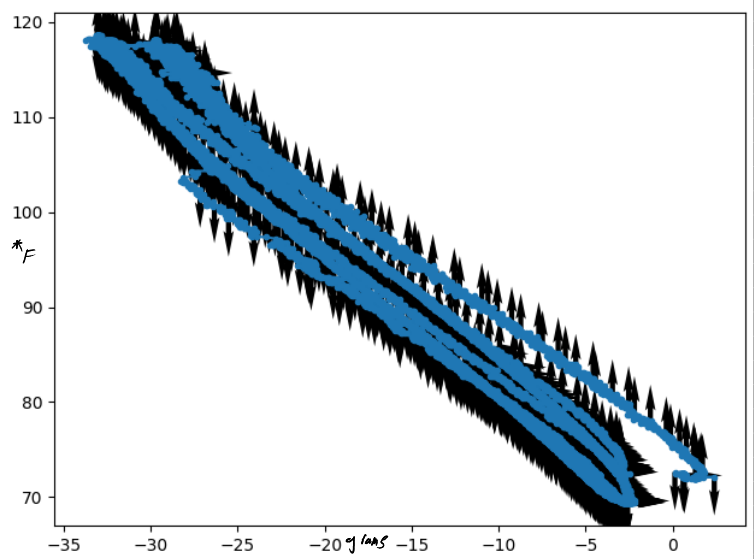
#15: Mass & Temperature Single-ended Shear Beam Load Cell

The following fixture was constructed and placed on a 3D printer heat bed for thermal conditioning testing. The probe was taped to the non-load bearing side of the load cell with copper tape to try to thermally couple the two.

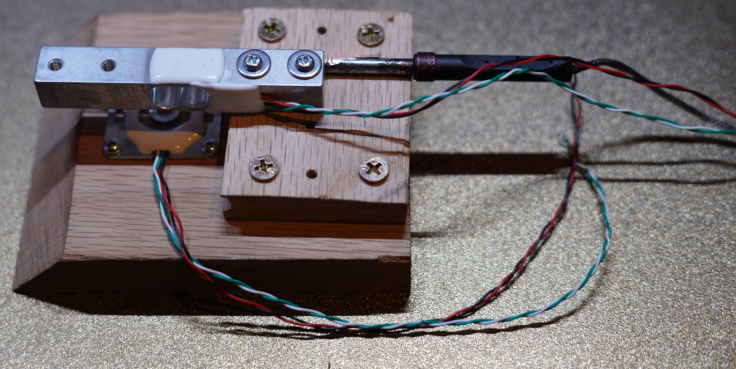
The fixture was thermally cycled between [70, 120] *F, approximately, three times.

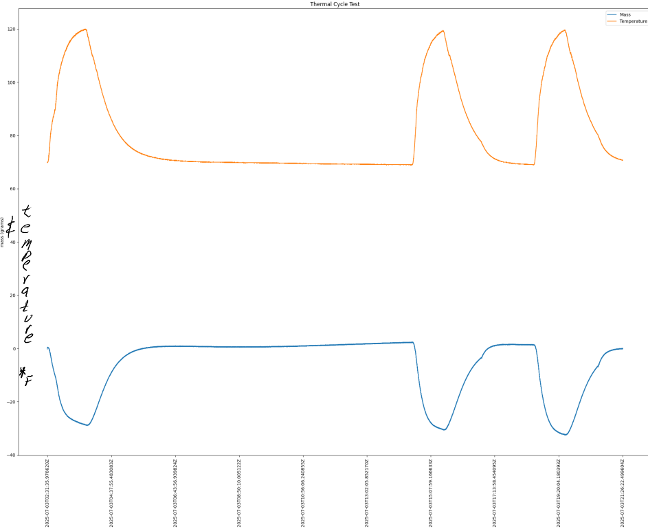
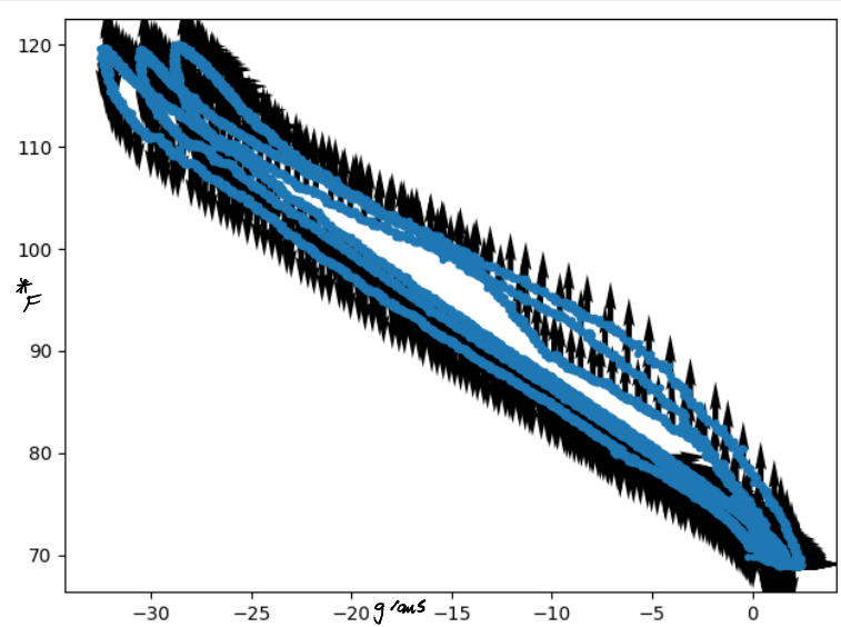
The total drift in mass was [2, -31] grams. There was hysteresis when going up/down in temperature. The width of the hysteresis was approximately 5-7 grams.

The same test was performed, this time with a 798 gram load using quarters and coffee coasters. The intent is to see if the load cell responds to temperature differently when loaded.

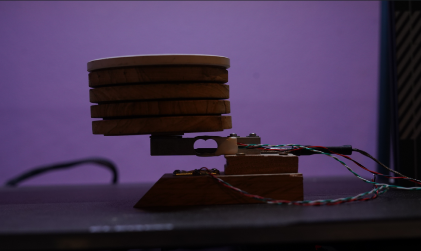
The fixture was thermally cycled between [70, 120] *F, approximately, three times.

The total drift in mass observed was again, about [2,-32] grams. The width of the hysteresis about 5-7 grams.

Summary:

The single-ended shear beam load cell responds to environmental temperature in a more predictable way than the planar load cell. This is likely due to complexities introduced in the strain field by multiple axis of warping in the planar cell. The shear beam has a simpler strain field that is more predictable with temperature changes.

I am wondering how much of the non-repeatable, unpredictable, non-linearities could be eliminated with a thermistor embedded into the metal of the load cell. The thermal response of the probe and the load cell are likely different. In this experiment, they were marginally thermally coupled using copper tape.

From these findings, the Growbies effort is going to shift to implementing a single-ended shear beam with an integrated thermistor. Temperature correction will be made. This will provide lower thermal drift error rates. This is important when trying to keep track of a plant growing in a container over long periods of time with varying environmental temperatures.

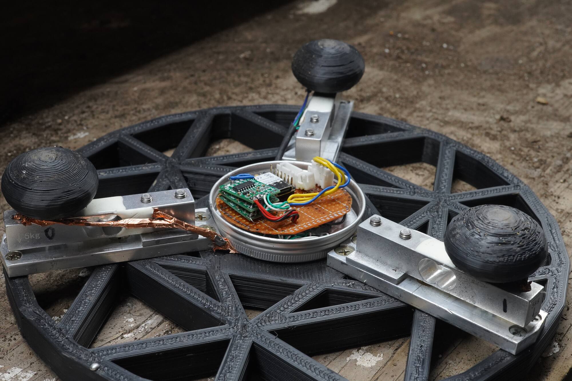
Prototype #3

The mechanics:

• 10” circle

• shear beam load cells with aluminum mounts

• 3D printed PLA

The electronics:

• esp32c3

• FTDI 232RL USB <-> UART

• 4x HX711

Testing

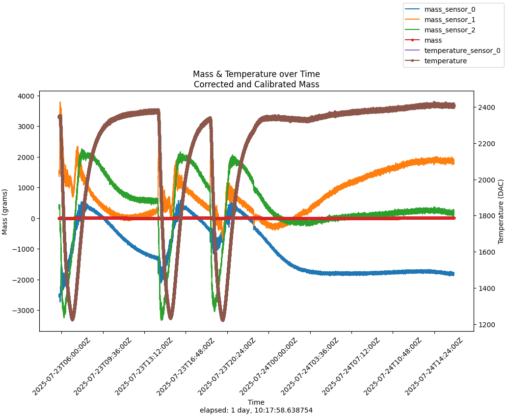
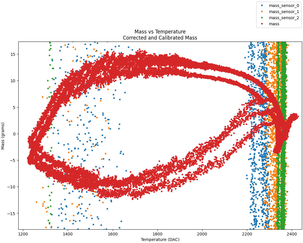
#1: Corrected and Calibrated Zero Offset Drift

Here is a thermal test of the prototype after it has been temperature corrected and calibrated. The units are a bit confusing on the plot. The individual mass sensors are in units of DAC. The red, mass total, is in units of grams.

The thermistors are in units of DAC. This test is varying the temperature through the range of [25*C, 65*C] approximately.

Here we can see the temperature varying over time and the per sensor mass varying with temperature.

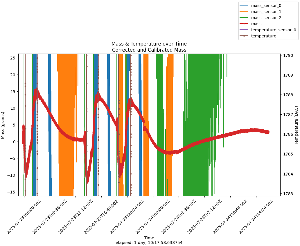
Here is a zoomed in (y-axis) to see how much the total mass is drifting during the course of the thermal cycling. Approximately +/- 15 grams.

This is another look at the same data. This time mass is plotted against temperature. We see that there is hysteresis in the per sensor mass output.

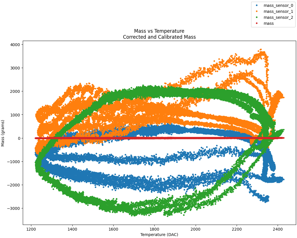
A zoomed in view of above. Again, we see approximately +/- 15 grams of error corrected and calibrated mass.

Growing

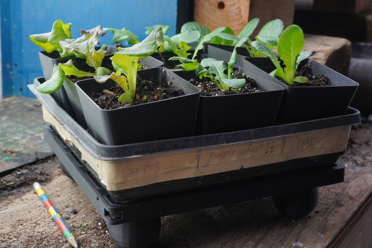
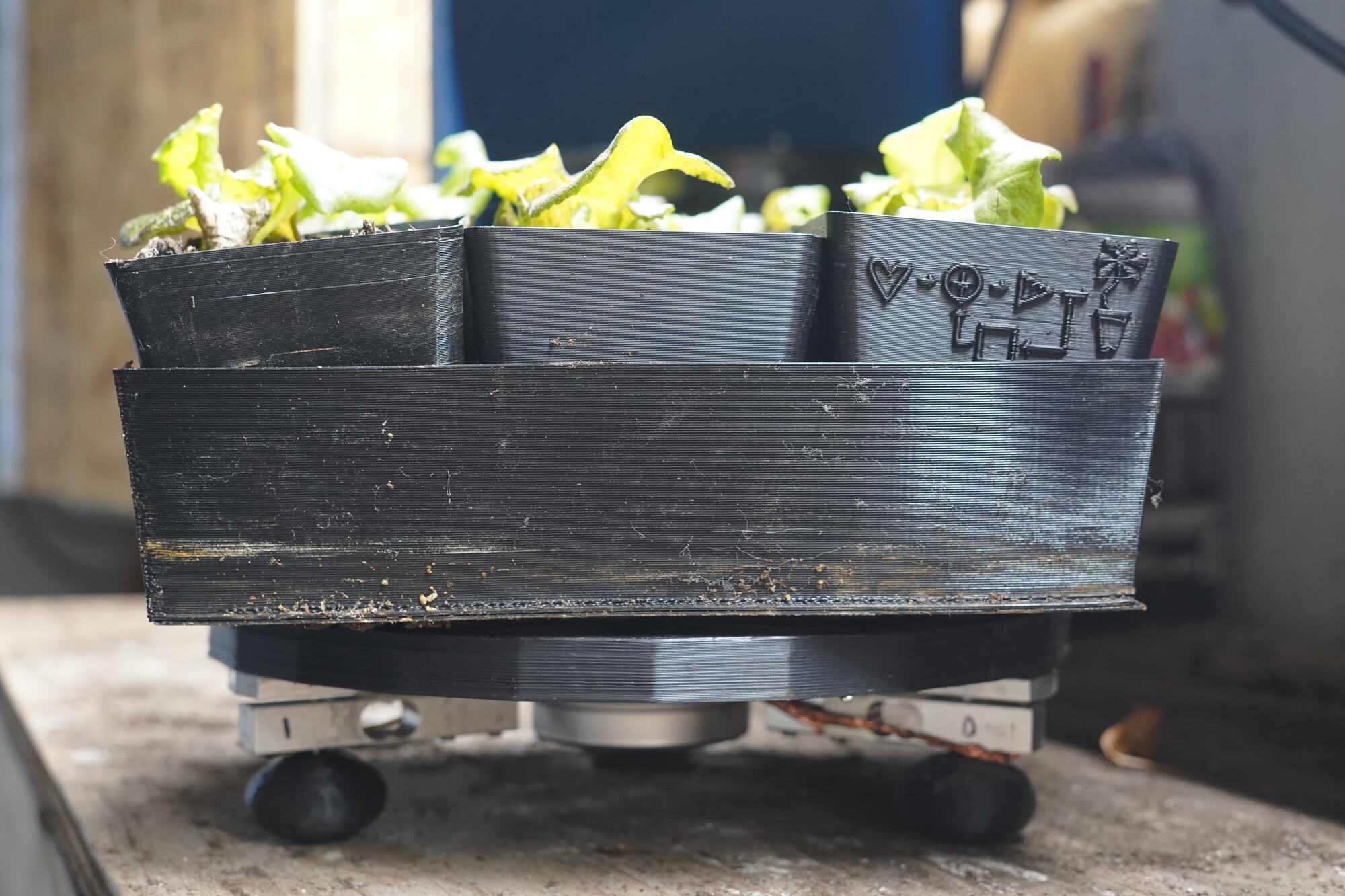
#1: 10” x 10” tray of lettuce

In this experiment, lettuce will be grown on top of the device for continuous data collection.

Shown below is the setup. This was taken mid-experiment.

Shown below is mass & temperature over time. There is lots of noise on temperature sensor 2 with fluorescent lights. Then, the noise is reduced on transition to LED lights. Sensor 2 did not have shielding on the single-ended thermistor wiring. It is interesting to see the susceptibility to noise and the reduction with shielding.

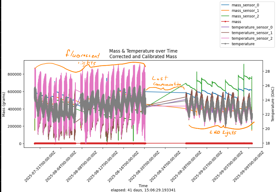
The end result of this experiment was, sadly, that the entire tray of lettuce died. Heh, I wish I had taken a picture, but I was annoyed enough to not think of it…:)

Anyways, I think the plant got overwhelmed with light on transition to LEDs. I went from 8 fluorescent tubes, to 8 led tubes. Since this experiment, I have reduced the length of light and the quantity of light. Now the plants are much happier.

Additionally, we were out of town for a few days around the time of the communication outage. This, combined with the lighting misconfiguration was more than the poor lettuce plants could handle.

Here is a zoomed in version of the above plot, focusing only on total mass.

Even though the results were not what I was hoping for (great lettuce), there is value here. From the data we better understand where things started to go poorly from the association made with the data.

I hope that the data growbies collects and the analysis thereof will help solve problems like these.